High-dimensional quantile regression using boosting. This repository is the official implementation of …
TODO: Add Article from arXiv when available
Quantile Regression is a popular tool to model the conditional quantiles of a response variable. In a high-dimensional setting, the theoretical results are largely limited to a penalized quantile regression model (Belloni and Chernozhukov, 2011).
Instead, we employ a greedy procedure to gradually improve the regression function. To overcome the non-differentiability of the check loss funciton, we employ the convolution-type smoothed quantile regression (Fernandes, Guerre and Horta, 2019 and He, Pan, Tan, Zhou).
Installation qboost
To install development version from GitHub, run the following commands:
# install.packages("devtools")
remotes::install_github("SvenKlaassen/qboost")
Introduction to Quantile Regression
In quantile regression the conditional \(\tau\)-quantile of some response variable \(Y\) is fitted. Here, we assume the conditional quantile \[F_{Y|X}^{-1}(\tau|x)=x^T\beta_\tau\] to be a linear function of the covariates. It can be shown \[\beta_\tau = \arg\min_{\beta\in\mathbb{R}^p}\mathbb{E}[\rho_\tau(Y - X^T\beta)],\] where \[\rho_\tau(x) = (\tau - I_{\{x\le 0\}})x\] is the check function (Quantile Regression).
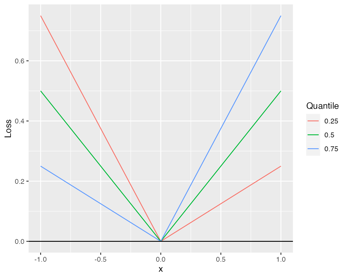 Since the loss function is nondifferentiable at zero, the theoretical results rely on a smoothed version of the loss, based on a kernel density estimator. Given a symmetric kernel \(k:\mathbb{R}\to [0,\infty)\) and a bandwidth \(h\), the smoothed loss is defined as the convolution \[\rho_{\tau,h}(x):=(\rho_\tau*k_h)(x)=\int_{-\infty}^\infty\rho_\tau(y)k_h(y-x)dy\] with \(k_h(x)=(1/h)k(x/h)\).
In the plot you can see different examples using different kernels (all with bandwidth \(h = 0.1\)). 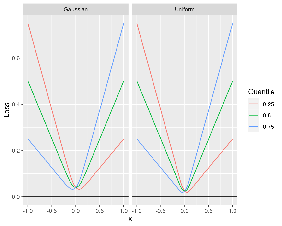
The difference to the desired loss function \(\rho_\tau\) is the largest at the origin.
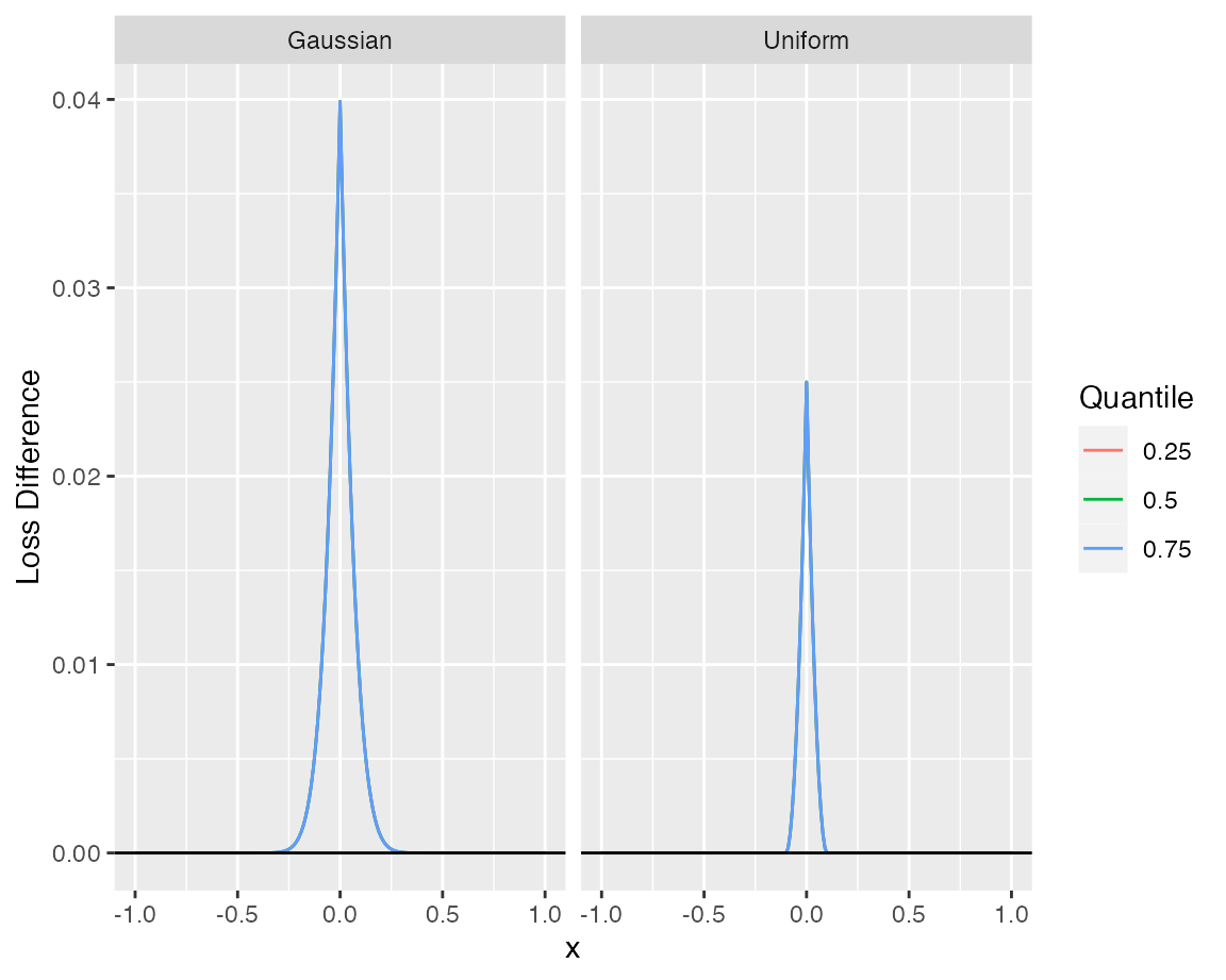 In the figure one can see that the difference behaves uniformly over different quantiles.
The quantile boosting algorithm applies greedy algorithms to minimize the corresponding loss functions.
Quantile Boosting: Example
We generate data from a basic linear model \[ Y = \beta_0 + X^T\beta +\epsilon,\] where \(\beta_0=1\) and \(\epsilon\sim t_2\). To account for a high-dimensional setting, we only generate \(n = 200\) observations, whereas the covariates \(X\) are generated from a standard multivariate gaussian distribution of dimension \(p = 500\). The coefficient vector is set to \[ \beta_j = \begin{cases} 1,\quad j = 1,\dots s\\ 0,\quad j = s+1,\dots,p\end{cases},\] such that the first \(s\) components are relevant.
library(MASS)
set.seed(42)
n <- 200; p <- 500; s <- 4
beta <- rep(c(1,0),c(s+1,p-s))

X = mvrnorm(n, rep(0, p), diag(p))
epsilon = rt(n, 2)
Y = cbind(1, X) %*% beta + epsilon

n_test <- 1000
X_test = mvrnorm(n_test, rep(0, p), diag(p))
epsilon_test = rt(n_test, 2)
Y_test = cbind(1, X_test) %*% beta + epsilon_test
Orthogonal Quantile Boosting/ Weak Chebyshev Greedy Algorithm (WCGA)
We start with the orthogonal variant of the qboost algorithm (WCGA, by setting stepsize = NULL) and proceed for \(100\) greedy selection steps.
library(qboost)
n_steps <- 100; tau <- .5
model_WCGA <- qboost(X,Y, tau = tau, m_stop = n_steps, h = 0.2, kernel = "Gaussian", stepsize = NULL)
# selected covariates
print(model_WCGA$selection_path[1:10])
#>  [1]   3   1   2   4 410 343 433 422 132  12
# predict values
print(head(predict(model_WCGA, newdata = X_test)))
#> 6 x 1 Matrix of class "dgeMatrix"
#>        Step_100
#> [1,]  1.2519807
#> [2,]  7.1507897
#> [3,] -1.9682364
#> [4,]  0.3923533
#> [5,]  3.0006988
#> [6,]  3.9602882
At first let us take a look at the Loss
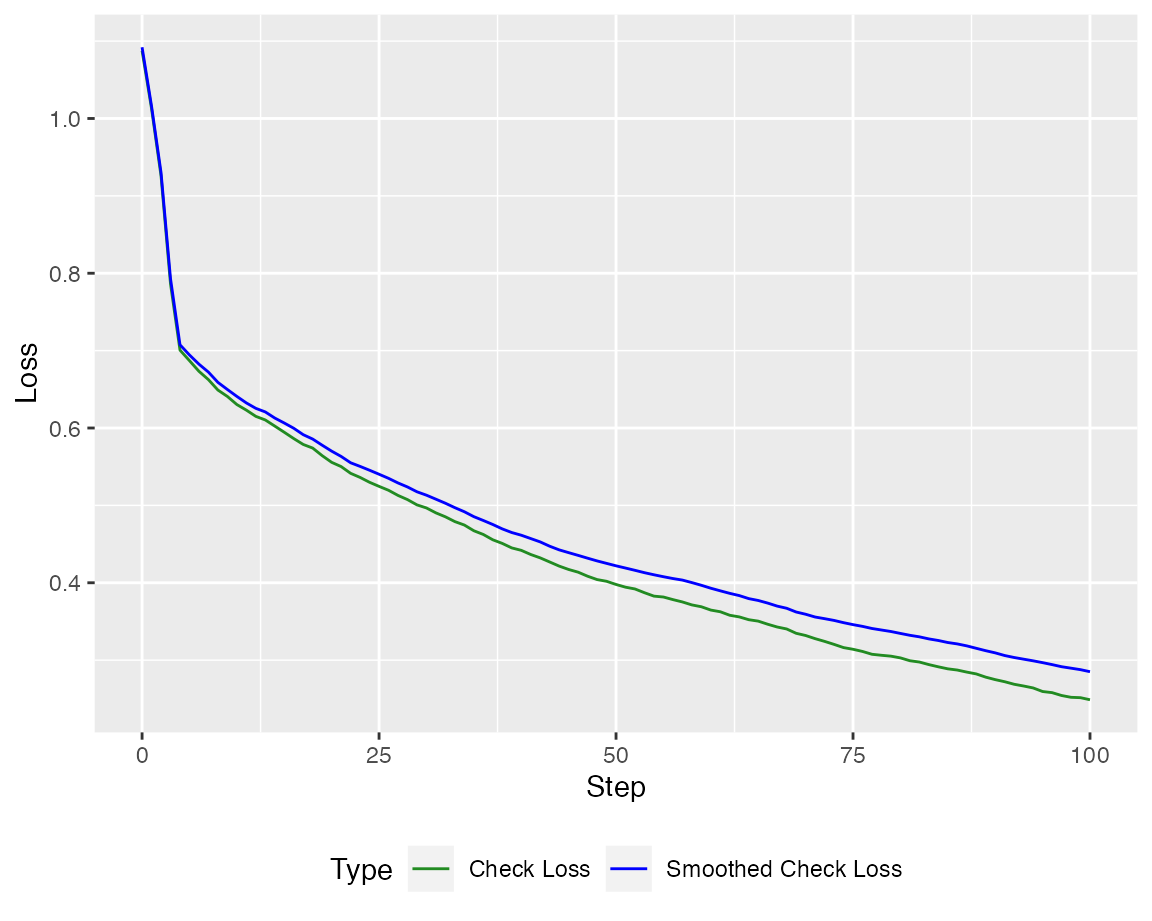
Of course, the loss is much more interesting on a test set.
autoplot(model_WCGA, new_Y = Y_test, newdata = X_test)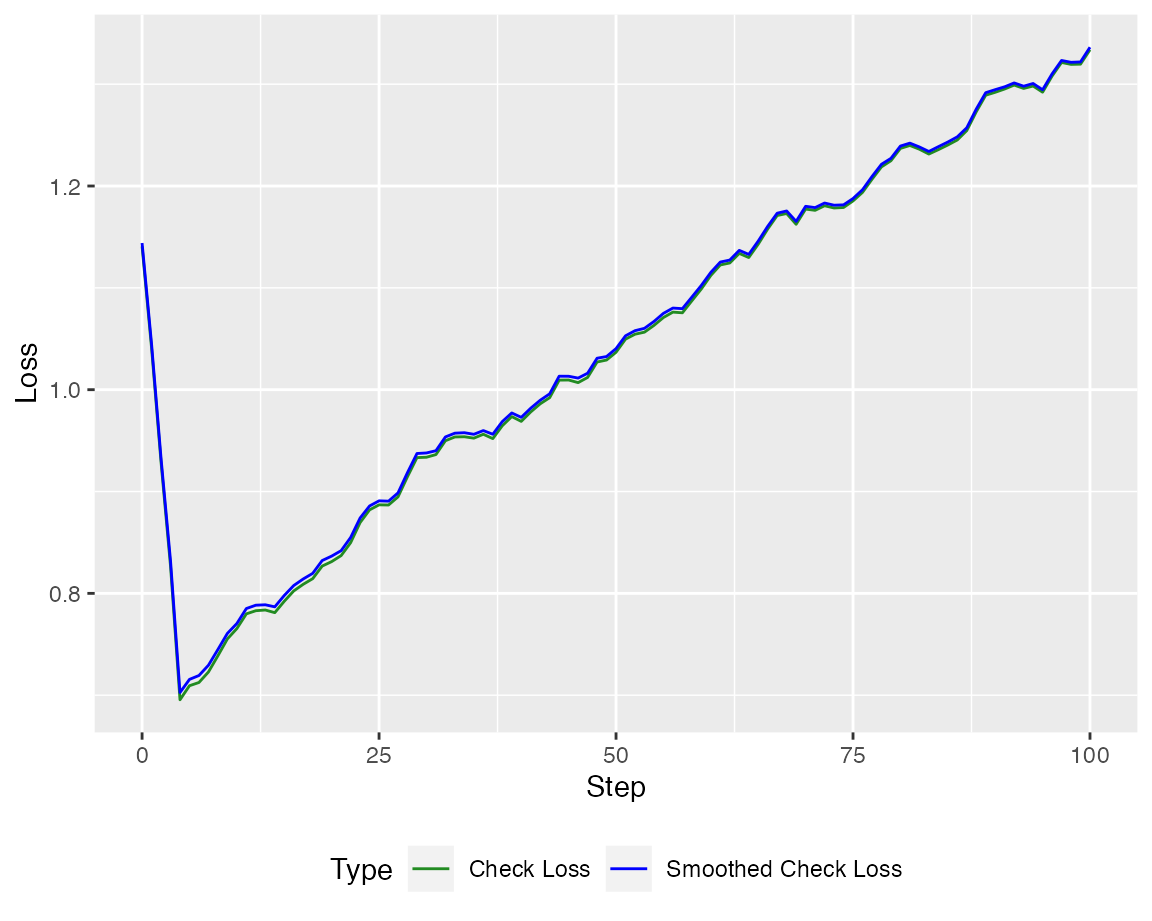
Quantile Boosting / Weak Greedy Algorithm (WGA, shortened)
Additionally, we can employ the Weak Greedy Algorithm (here with \(400\) steps).
n_steps_WGA <- 400
model_WGA <- qboost(X,Y, tau = tau, m_stop = n_steps_WGA, h = 0.2, kernel = "Gaussian", stepsize = 0.1)
Again, the loss is minimized
autoplot(model_WGA, new_Y = Y, newdata = X)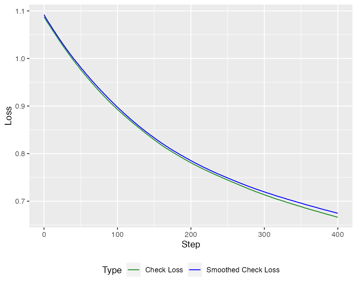
but we have to find the right stopping criterion to minimize the out of sample loss.
autoplot(model_WGA, new_Y = Y_test, newdata = X_test)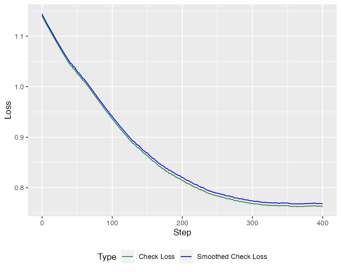
Crossvalidation
To have a reasonable stopping criterion, a crossvalidated version of the algorithms is implemented. At first, lets take a look at the orthogonal variant
cv_model_WCGA <- cv_qboost(X,Y, tau = tau, m_stop = n_steps,
                           h = 0.2, kernel = "Gaussian", stepsize = NULL)
autoplot(cv_model_WCGA, new_Y = Y_test, newdata = X_test)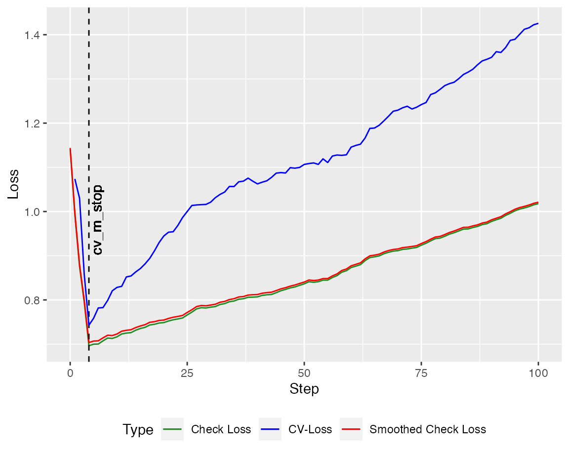
Next, repeat the same for the non-orthogonal algorithm.
cv_model_WGA <- cv_qboost(X,Y, tau = tau, m_stop = n_steps_WGA,
                           h = 0.2, kernel = "Gaussian", stepsize = 0.1)
autoplot(cv_model_WGA, new_Y = Y_test, newdata = X_test)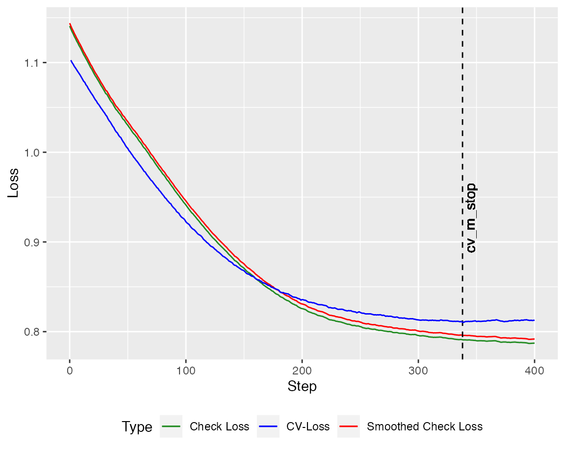
To compare the performance to the oracle model (here in green), we apply the conquer algorithm to the first \(s\) components of \(X\) and report the loss on the test set.
library(conquer)
fit_conquer <- conquer(X[,1:s], Y, tau = tau, h = 0.2, kernel = "Gaussian")
resid_conquer <- Y_test - cbind(1,X_test[,1:s])%*%fit_conquer$coeff
loss_conquer <- smooth_check_loss(resid_conquer,tau = tau, kernel = NULL)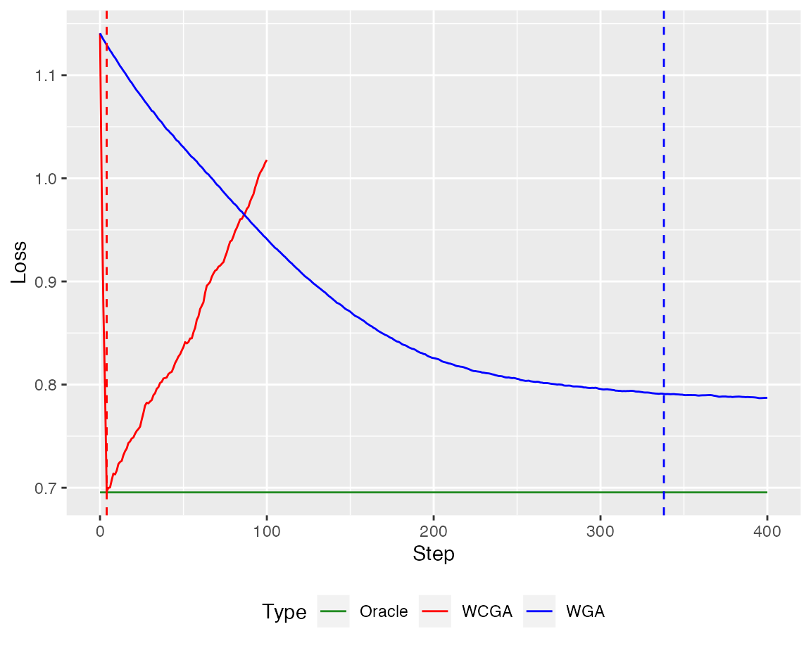
References
He, Xuming, et al. “Smoothed quantile regression with large-scale inference.” arXiv preprint arXiv:2012.05187 (2020). Paper
Belloni, Alexandre, and Victor Chernozhukov. “ℓ1-penalized quantile regression in high-dimensional sparse models.” The Annals of Statistics 39.1 (2011): 82-130. Paper
Fernandes, Marcelo, Emmanuel Guerre, and Eduardo Horta. “Smoothing quantile regressions.” Journal of Business & Economic Statistics 39.1 (2021): 338-357. Paper