qboost - Get Started • qboost

Installation

To install development version from GitHub, run the following commands:

# install.packages("devtools")
remotes::install_github("SvenKlaassen/qboost")

A simple Example

We generate data from a basic linear model \[ Y = \beta_0 + X^T\beta +\epsilon,\] where \(\beta_0=1\) and \(\epsilon\sim t_2\). To account for a high-dimensional setting, we only generate \(n = 200\) observations, whereas the covariates \(X\) are generated from a standard multivariate gaussian distribution of dimension \(p = 500\). The coefficient vector is set to \[ \beta_j = \begin{cases} 1,\quad j = 1,\dots s\\ 0,\quad j = s+1,\dots,p\end{cases},\] such that the first \(s\) components are relevant.

library(MASS)
set.seed(42)
n <- 200; p <- 500; s <- 4
beta <- rep(c(1,0),c(s+1,p-s))

X = mvrnorm(n, rep(0, p), diag(p))
epsilon = rt(n, 2)
Y = cbind(1, X) %*% beta + epsilon

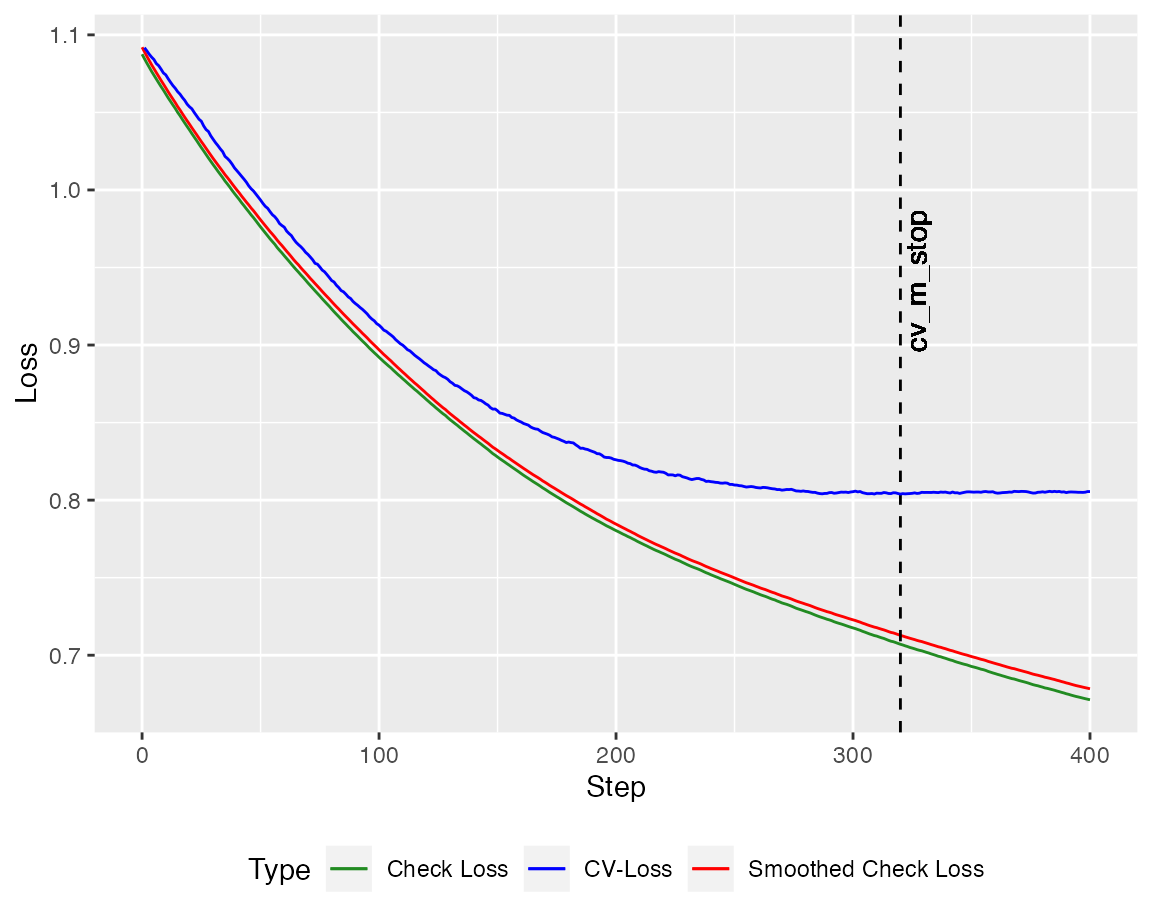
We can employ the crossvalidated version of the quantile boosting algorithm (here with \(400\) steps). The autoplot method plots the crossvalidated loss against the check loss (and the smoothed version). Here, the loss is calculated on the training set.

library(qboost)
library(ggplot2)
model <- cv_qboost(X,Y, tau = 0.5, m_stop = 400,
                   h = 0.2, kernel = "Gaussian", stepsize = 0.1)
autoplot(model, new_Y = Y, newdata = X)

To predict new values one can use the predict method.

head(predict(model, newdata = X))
#> 6 x 1 Matrix of class "dgeMatrix"
#>        Step_320
#> [1,]  1.0553096
#> [2,]  2.6283815
#> [3,] -0.1195155
#> [4,]  0.4163286
#> [5,]  1.1185732
#> [6,]  2.4744881

For the crossvalidated version the prediction is based on the Step with the smallest crossvalidated loss. This can be adjusted manually

head(predict(model, newdata = X, step = 0))
#> 6 x 1 Matrix of class "dgeMatrix"
#>        Step_0
#> [1,] 1.115022
#> [2,] 1.115022
#> [3,] 1.115022
#> [4,] 1.115022
#> [5,] 1.115022
#> [6,] 1.115022