DoubleMLDeep: Estimation of Causal Effects with Multimodal Data

Causal Inference and Missing Data Group at Inria
22.04.2024

Sven Klaassen
University of Hamburg
Economic AI

Jan Teichert-Kluge
University of Hamburg

Philipp Bach
University of Hamburg
Economic AI

Victor Chernozhukov
Massachusetts Institute
of Technology

Martin Spindler
University of Hamburg
Economic AI

Motivation

Motivation

• Causal Inference mainly relies on tabular data

• In a lot of applications additional unstructured data is available

• We consider multimodal data as confounders
• Applications in Marketing, Medicine / Health, Finance, ….
  • Price elasticity of demand
  • Estimation of treatment effects conditioning on X-ray images

Motivating Example - PLR

Partially linear regression model (PLR)

\[ \begin{align} Y &= \theta_0 D + g_0(X) + \varepsilon, & \mathbb{E}[\varepsilon | X, D] = 0 \label{eq:plr1} \\ D &= m_0(X) + \vartheta, & \mathbb{E}[\vartheta | X] = 0 \label{eq:plr2} \end{align} \]

with

• \(Y\) - outcome variable
• \(D\) - policy/treatment variable
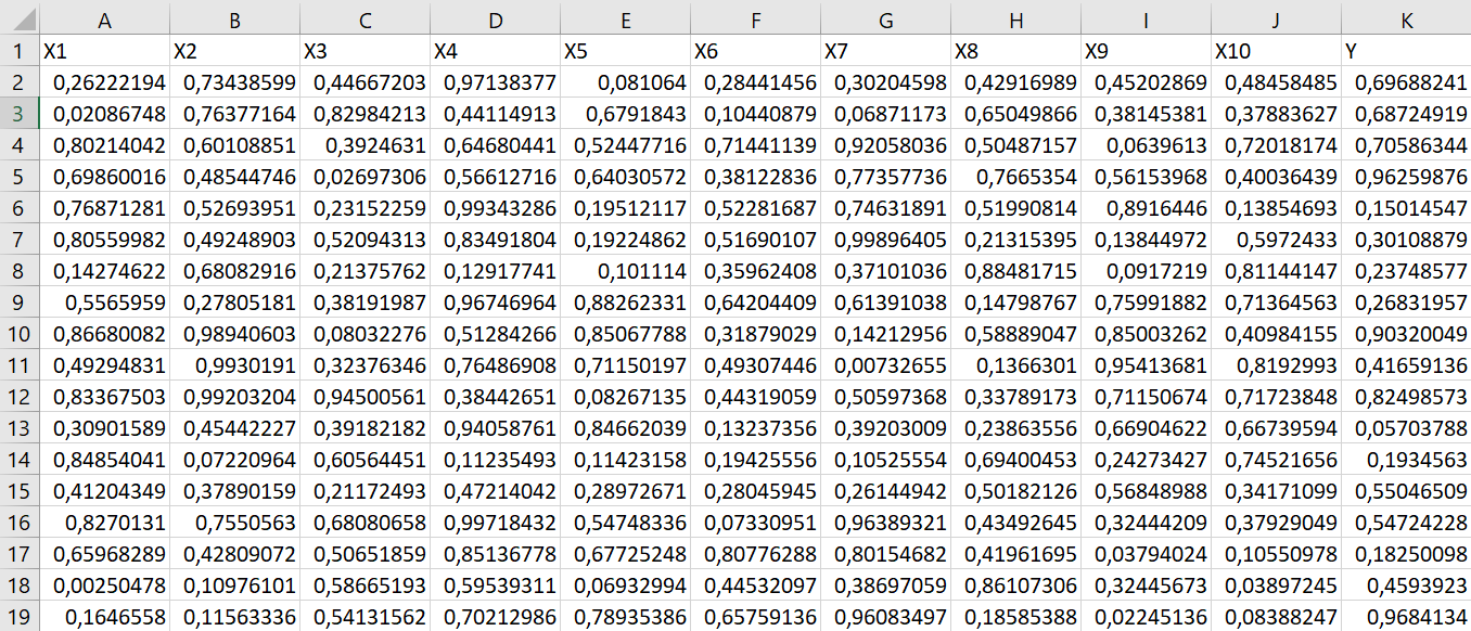
• \(X = (X_1, \dots)^T\) - vector of additional controls
• \(\varepsilon\), \(\vartheta\) - stochastic errors

DAG for PLR Model

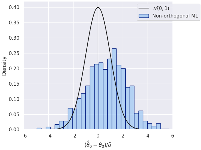
Motivating Example - Regularization Bias

• What if we simply plug-in ML predictions \(\hat{g}(X)\) for \(g_0(X)\) into \(Y = \theta_0D + g_0(X) + \varepsilon\)?

Motivating Example - Orthogonalization

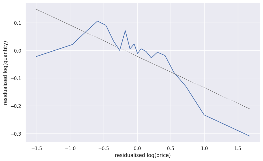
• Frisch-Waugh-Lovell style approach: \(\theta_0\) can be consistently estimated by partialling out \(X\), i.e,

  1. Predict \(Y\) and \(D\) by \(\mathbb{E}[Y|X]\) and \(\mathbb{E}[D|X]\), obtained using ML methods
  2. Residualize \(\tilde{Y} = Y - \mathbb{E}[Y|X]\) and \(\tilde{D} = D - \mathbb{E}[D|X]\)
  3. Regress \(\tilde{Y}\) on \(\tilde{D}\) to obtain \(\hat{\theta}\)

Double/Debiased Machine Learning (DML)

• Use machine learning methods to fit \[ \begin{align*} l_0(X)&:=\mathbb{E}[Y|X]\\ m_0(X)&:=\mathbb{E}[D|X] \end{align*} \]
• Construct the orthogonalized score (either cross-fitting or split the sample) for a fitted nuisance learner \(\hat{\eta}:=(\hat{l}, \hat{m})\) \[ \psi(W,\theta,\hat{\eta}) := \Big(Y - \hat{l}(X) - \theta\big(D-\hat{m}(X)\big)\Big)\Big(D-\hat{m}(X)\Big) \]
• Compute the estimate as the solution of \[ 0 = \frac{1}{n}\sum_{i=1}^n \psi(W,\hat{\theta},\hat{\eta}) \]

Double/Debiased Machine Learning (DML)

• Neyman Orthogonality \[ \left.\partial_\eta \mathbb{E}[\psi(W; \theta_0, \eta)] \right|_{\eta=\eta_0} = 0 \] ensures that the moment condition identifying \(\theta_0\) is insensitive to small pertubations of the nuisance function \(\eta\) around \(\eta_0\)

• Assumptions for the nuisance elements (see Chernozhukov et al. (2018)) \(\lVert \hat{m} - m_0 \rVert_{P,2} \times \big( \lVert \hat{m} - m_0 \rVert_{P,2} + \lVert \hat{\ell} - \ell_0\rVert _{P,2}\big) \le \delta_N N^{-1/2}\)

• Under some regularity conditions the estimator \(\hat{\theta}\) concentrates in \(1/\sqrt{n}\)-neighborhood of \(\theta_0\) and \[ \sqrt{n}(\hat{\theta} - \theta_0) \to \mathcal{N}(0,\sigma^2) \]

\(\Rightarrow\) simple approach to control for confounders, if they can be used for ML models!

DoubleML Deep

DoubleML Deep - Motivation

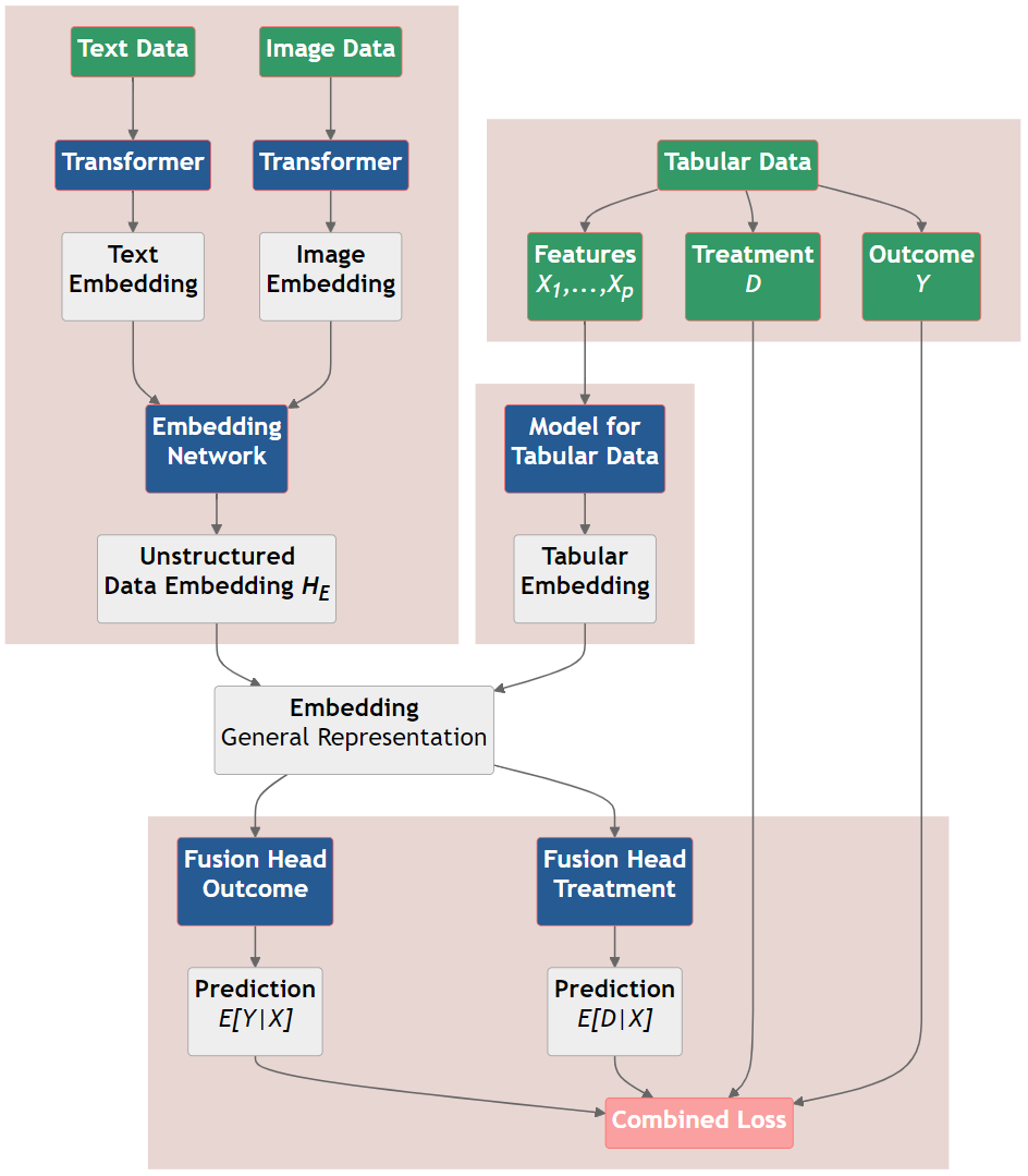
• Use multimodal data (text and images) additionally to conventional tabular features

Examples of directed acyclic graphs (DAGs) with image and text confounding. (a) Direct confounding via image, text and tabular data. (b) Treatment decision is driven by text and images. All backdoor paths are blocked by conditioning on both image and text data.

DoubleML Deep - Module Structure

High-Level PLR Model Architecture. Both nuisance components are trained simultaneously with a combined loss.

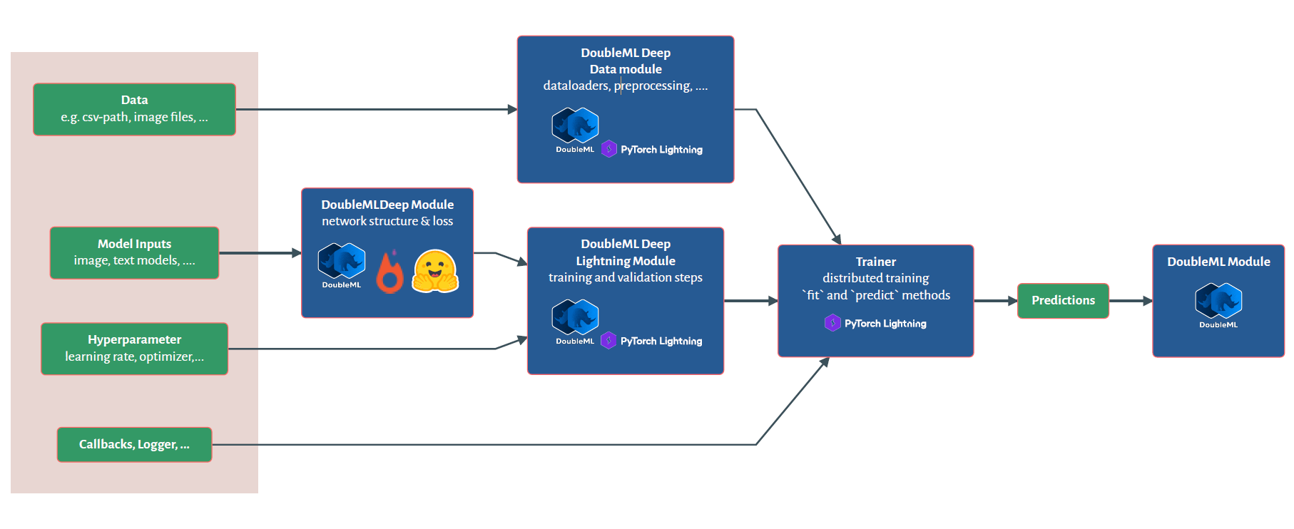
DoubleML Deep - Workflow

High-Level Workflow of DoubleMLDeep

Now I would like to briefly explain the workflow of DoubleMLDeep in Python. wor First of all, some necessary input parameters must be defined. Then the actual DoubleMLDeep network can be created, which uses Hugging Face Transformer models and the Pytorch framework, among other things.

A DoubleMLDeep Data Module must be created and handles the various input data such as texts and images. This uses the Pytorch Lightning Framework.

The DoubleMLDeep Lightning Module also uses Pytorch Lightning and contains additional training parameters.

The network can now be trained with the pytorch Lightning Trainer. The corresponding predictions in the DoubleML package can then be used to obtain the estimate of the causal parameter.

DoubleML Deep - More Details

• Use pretrained models for unstructured data e.g. Bert and Beit

• Basic models for tabular data seem sufficient

• Monitor the nuisance losses

  • \(\lVert Y - \hat{l}(X) \rVert_{P,2} \le \lVert l_0(X) - \hat{l}(X) \rVert_{P,2} + \sigma_{\epsilon}\)
  • \(\lVert D - \hat{m}(X) \rVert_{P,2} \le \lVert m_0(X) - \hat{m}(X)\rVert_{P, 2} + \sigma_{\vartheta}\)

• Unstructured Data Models: We employ pre-trained models like BERT and BEiT to extract valuable information from unstructured data, including product descriptions and images.

• Tabular Data Models: Basic models for tabular data have proven to be effective.

• Monitoring Nuisance Losses: To ensure the reliability of our estimations, we diligently monitor nuisance losses. The following conditions are crucial for assessing the quality of our models:

  • \(\lVert Y - \hat{l}(X) \rVert_{P,2} &\le \lVert l_0 - \hat{l}(X) \rVert_{P,2} + \sigma_{\epsilon}\)

  • $ D - (X) {P,2} &m_0(X) - (X){P,2} + _{}$

  These conditions help maintain the validity of our estimates by ensuring that the discrepancies between our estimated nuisance functions and their true counterparts, along with stochastic errors, remain within acceptable bounds.

Semi-Synthetic Data

Original Datasets

• We generate a semi-synthetic dataset with a known treatment effect parameter

• To generate credible confounding wil be based on the labels or outcomes of the corresponding supervised learning task

• We use the following datasets:

Modality	Dataset	Target \(\tilde{X}\)	Control \(X\)
Tabular	DIAMONDS Wickham (2016)	\(\log(\text{Price})\)	Carat, Cut, Color, Clarity, …
Text	IMDB Maas et al. (2011)	Sentiment	Review Text
Image	CIFAR-10 Krizhevsky (2009)	Label	Image

…

Data Generating Process

We generate a semi-synthetic dataset according to the underlying PLR model \[ \begin{align} Y &= \theta_0 D + \tilde{g}_0(\tilde{X}) + \varepsilon, \\ D &= \tilde{m}_0(\tilde{X}) + \vartheta, \end{align} \] where \(\tilde{X}= (\tilde{X}_{\text{tab}}, \tilde{X}_{\text{txt}}, \tilde{X}_{\text{img}})\) with the following additive structure \[ \begin{align} \tilde{g}_0(\tilde{X}) &= \sum_{\text{mod}\in\{\text{tab},\text{txt},\text{img}\}} \tilde{g}_{\text{mod}}(\tilde{X}_{\text{mod}}) \\ \tilde{m}_0(\tilde{X}) &= \sum_{\text{mod}\in\{\text{tab},\text{txt},\text{img}\}} \tilde{m}_{\text{mod}}(\tilde{X}_{\text{mod}}) \end{align} \] and \(\varepsilon, \vartheta \sim \mathcal{N}(0, 1)\).

…

Data Generating Process

• The effect on the outcome \(Y\) is generated via a standardized version of target variable to balance the confounding impact of all modalities: \[ \begin{align} \tilde{g}_{\text{mod}}(\tilde{X}_{\text{mod}}) = \frac{\tilde{X}_{\text{mod}} - \mathbb{E}[\tilde{X}_{\text{mod}}]}{\sigma_{\tilde{X}_{\text{mod}}}}, \quad \text{mod}\in\{\text{tab}, \text{txt}, \text{img}\} \end{align} \]

• Further, to ensure a strong confounding, the impact on the treatment \(D\) is defined via: \[ \begin{align} \tilde{m}_{\text{mod}}(\tilde{X}_{\text{mod}}) = -\tilde{g}_{\text{mod}}(\tilde{X}_{\text{mod}}), \quad \text{mod}\in\{\text{tab}, \text{txt}, \text{img}\} \end{align} \]

• The treatment effect is set to \(\theta_0=0.5\) with \(n=50.000\) samples in the dataset

• Both \(\tilde{g}_0(X)\) and \(\tilde{m}_0(X)\) are rescaled to ensure a signal-to-noise ratio of \(2\) for \(Y\) and \(D\) (given unit variances of the error terms)

…

Challenges

• Dependency on the target of the modality \(\tilde{X}_{\text{mod}}\)
  • Might not be fully explained by the corresponding features \(X_{\text{mod}}\)
  • E.g. price of diamonds can not be fully explained by the carat, cut, color, etc.
• Consequently, the estimate \(\hat{\theta}\) might only be able to account for the part of confounding which can be explained by the input features: \[ \begin{align} \tilde{X}_{\text{mod}} = \mathbb{E}[\tilde{X}_{\text{mod}}|X_{\text{mod}}] + U_{\text{mod}}, \end{align} \] where \(U_{\text{mod}}\) can not be controlled for

Challenges

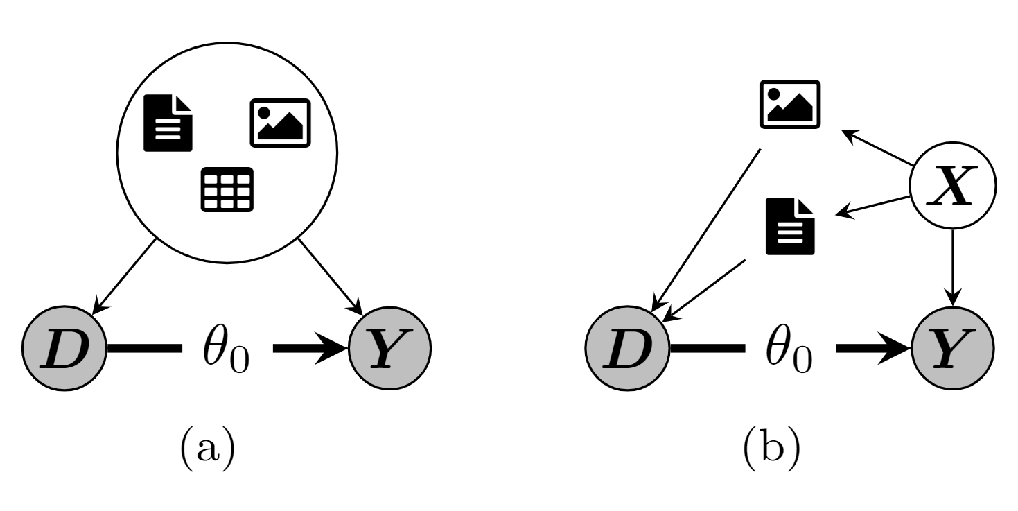
• Due to the negative sign and the additive structure, the confounding effect will ensure that higher outcomes \(Y\) occur with lower treatment values \(D\), creating a negative bias
• The independence of all three original datasets and the additive negative confounding results in a negative bias even if we only control for a subset of confounding factors

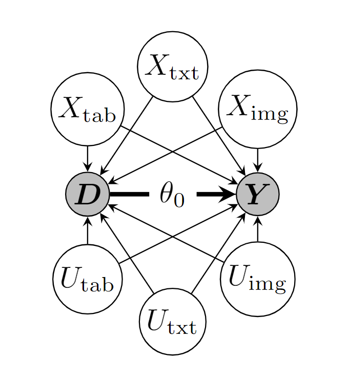
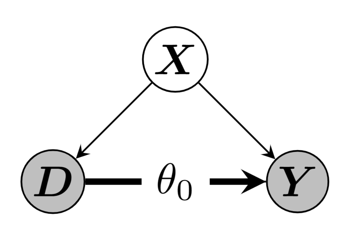
DAG for the semi-synthetic dataset. The confounding via the features \(X=(X_{\text{tab}}, X_{\text{txt}}, X_{\text{img}})\) can be adjusted for, whereas the unexplained/noise parts \(U=(U_{\text{tab}}, U_{\text{txt}}, U_{\text{img}})\) are unobserved.

Bounds for the estimation of \(\theta_0\)

• Since all modalities contribute a negative bias, the semi-synthetic dataset can be used as a benchmark with an oracle upper bound of an effect estimate of \[ \theta_0=0.5 \]
• For the lower bound, one can not account for confounding at all and evaluate a basic ordinary least squares model with outcome \(Y\) on the treatment variable \(D\) (excluding all confounding variables) \[ \hat{\theta}_{\text{OLS}} = -0.4594 \]

Bounds for the estimation of \(\eta_0\)

• To access the predictive performance of the nuisance models, we can rely on oracle predictions of \[ \begin{align} \tilde{m}_0(\tilde{X}):= \mathbb{E}[D|\tilde{X}] \\ \tilde{l}_0(\tilde{X}):= \mathbb{E}[Y|\tilde{X}] &= \theta_0 \tilde{m}_0(\tilde{X}) + \tilde{g}_0(\tilde{X}) \end{align} \]
• Evaluating the oracle predictions \(\tilde{m}_0(\tilde{X})\) and \(\tilde{l}_0(\tilde{X})\) results in the following upper bounds for the performance of the nuisance estimators \[ \begin{align} R^2(D, \tilde{m}_0(\tilde{X})) &= 0.6713\\ R^2(Y, \tilde{l}_0(\tilde{X})) &= 0.5845 \end{align} \] on the whole dataset of \(n=50.000\) observations

Bounds for the estimation of \(\eta_0\)

• In order to compare the predictive performance of different models, a relative \(r^2\)-score with respect to the upper bound is defined as \[ \begin{align} 0 \leq r^2(D, \hat{m}) &:= \frac{R^2(D, \hat{m}(X))}{R^2(D, \tilde{m}_0(\tilde{X}))} \leq 1\\ 0 \leq r^2(Y, \hat{l}) &:= \frac{R^2(Y, \hat{l}(X))}{R^2(Y, \tilde{l}_0(\tilde{X}))} \leq 1 \end{align} \]

Models

• Baseline Model
  • Standard DML approach, relying only on tabular data \(X_{\text{tab}}\)
    
    
    
  • Based on the LightGBM package for estimation of the nuisance elements

• Deep Model
  • Uses the out-of-sample predictions of \(\hat{m}(X)\) and \(\hat{l}(X)\) generated from the model
    
    
  • Based on the RoBERTa Model for text modality, a VIT Model for images and a SAINT model for the tabular data

• Embedding Model
  • Generated embedding \(H_E\) is used together with the tabular features \(X_{\text{tab}}\) as input for LightGBM
  • Based on the RoBERTa Model for text modality, a VIT Model for images and a SAINT model for the tabular data

Simulation Results

Results of Simulation Study. Reported: mean ± sd. over five random train-test splits

	Baseline	Embedding	Deep
\(r^2(Y, \hat{l}_0)\)	\(0.31 \pm 0.01\)	\(0.87 \pm 0.02\)	\(\mathbf{0.90 \pm 0.01}\)
\(r^2(D, \hat{m}_0)\)	\(0.31 \pm 0.01\)	\(0.87 \pm 0.02\)	\(\mathbf{0.90 \pm 0.01}\)
\(\hat{\theta}\)	\(-0.32 \pm 0.01\)	\(\mathbf{0.28 \pm 0.01}\)	\(0.27 \pm 0.01\)

Higher = better (best in bold)

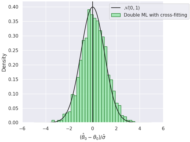
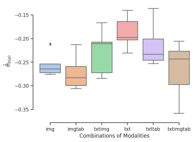
Simulation Results - Performance of \(\hat{\theta}\)

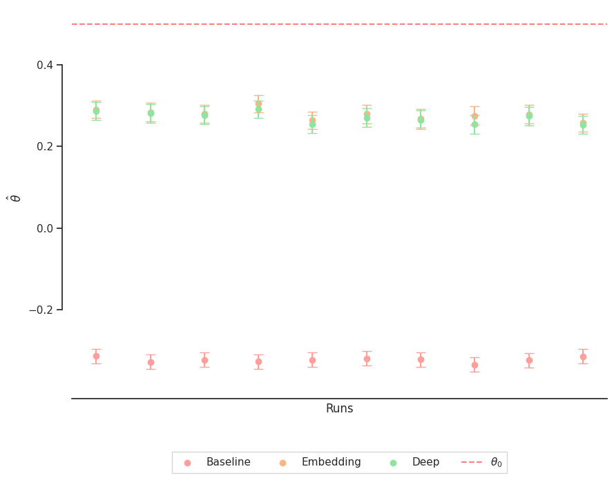
Boxplots of \(\hat{\theta}\). The Embedding Model and Deep Model have similar estimates. This indicates a stable and information-rich embedding \(H_E\), which provides a high explanatory contribution independent of the subsequent ML method for predicting \(Y\) and \(D\). \(\theta_0\) represents the upper bound.

Application

Application: Estimation of Price Elasticity

• Understanding price elasticity is crucial for economic analysis and business decisions
  • It influences strategies, pricing, and market dynamics
• Specifically in online marketplaces, unstructured data is available

Image Data

Text Data

Tabular Data

Amazon Toys Dataset

• Public Data from the Amazon sales platform from category toys and games for subcategories vehicles, cars and trucks.
• Using the Sales Rank as a proxy for quantities, as shown in Bajari et al. (2023).

Variable	Description
Sales Rank	Sales rank as weighted mean for the last 30 days
Price	Price as weighted mean for the last 30 days
Text	Combination of Title, Category, Description, etc.
Image	Image of the product

Amazon Toys Dataset

Continous Variables

• Reviews: Rating
  
• Reviews: Review Count
  
• New Offer Count: Current
  
• Count of retrieved live offers: New, FBA
  
• Count of retrieved live offers: New, FBM

Categorical Variables

• Lightning Deals: Upcoming Deal
  
• Buy Box: Is FBA

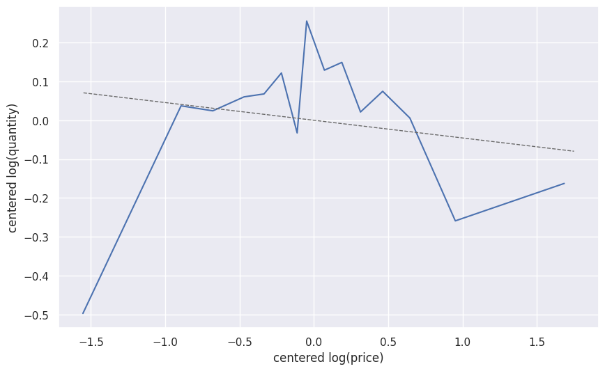
Scatterplots with OLS Regression of Tabular Variables and \(\ln(Q)\)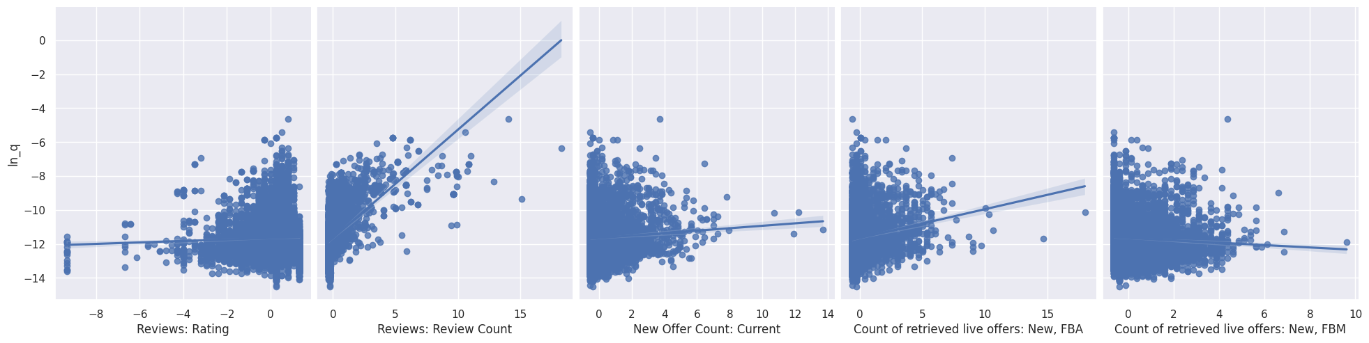

Model

• Run a simple log-log regression model
• Images and Text block backdoor path from price to demand (or sales rank)

\[ \ln(Q_{}) = \theta_0 \ln(P) + g_0(X) + \epsilon \]

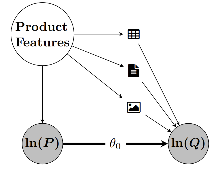
\(\Rightarrow\) The causal parameter \(\theta_0\) can be interpreted as price elasticity of demand!

Baseline OLS Model

• Baseline estimate with tabular covariates \(X_{\text{tab}}\)
• OLS: \[ \begin{align*} \ln(Q) =&\ \theta_0 \ln(P) + \beta^T X_{\text{tab}} + \epsilon \end{align*} \]
• \(R^2 = 0.330\)

2.5 %	\(\hat{\theta}\)	97.5 %
-0.072	-0.046	-0.019

Centered logarithmic negative sales rank over centered logarithmic price as binned plot

Baseline DML Model

• Estimate with tabular data as covariates \(X_{\text{tab}}\) in \(\texttt{DoubleMLPLR}\) model with \(\texttt{RandomForest}\) regressors
  • \(l_0(X_{\text{tab}}) := \mathbb{E}[\ln(Q)|X_{\text{tab}}]\)
    • \(R^2_{l_0} = 0.5986\)
  • \(m_0(X_{\text{tab}}) := \mathbb{E}[\ln(P)|X_{\text{tab}}]\)
    • \(R^2_{m_0} = 0.1884\)

2.5 %	\(\theta\)	97.5 %
-0.132	-0.1098	-0.080

Residualised logarithmic negative sales rank over residualised logarithmic price as binned plot

Deep Learning Models

• In this study, a variety of input data combinations were used to train \(\texttt{DoubleMLPLRDeep}\) models ¹:

Key	Used Confounders
\(\texttt{img}\)	\(X = (X_{img})\)
\(\texttt{imgtab}\)	\(X = (X_{img}, X_{tab})\)
\(\texttt{txtimg}\)	\(X = (X_{txt}, X_{img})\)
\(\texttt{txt}\)	\(X = (X_{txt})\)
\(\texttt{txttab}\)	\(X = (X_{txt}, X_{tab})\)
\(\texttt{txtimgtab}\)	\(X = (X_{txt}, X_{img}, X_{tab})\)

\(\Rightarrow\) The aim is to emphasize the benefits of utilizing unstructured data.

1. Subsequently, the top 5 performing instances for each combination were evaluated based on the minimum RMSE score of the validation data.

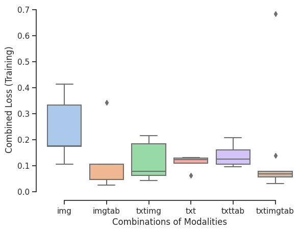
Deep Learning Models: RMSE-Scores

• Combined RMSE Score (Training)

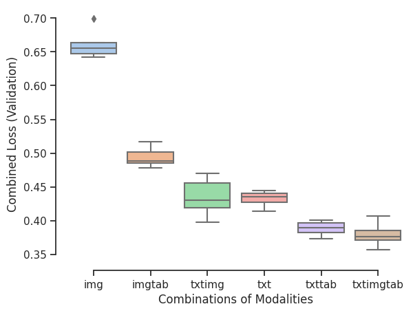
• Combined RMSE Score (Validation)

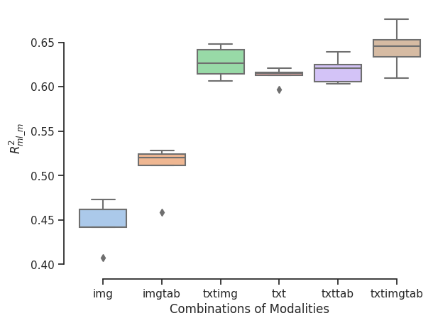
Deep Learning Models: \(R^2\)-Scores

• \(R^2\) of log(Quantity) on Validation Set

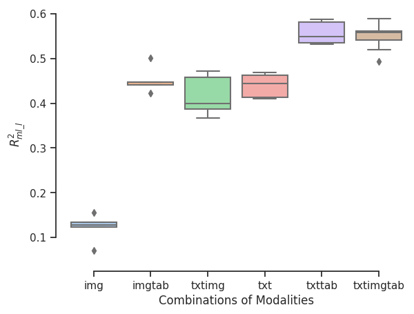
• \(R^2\) of log(Price) on Validation Set

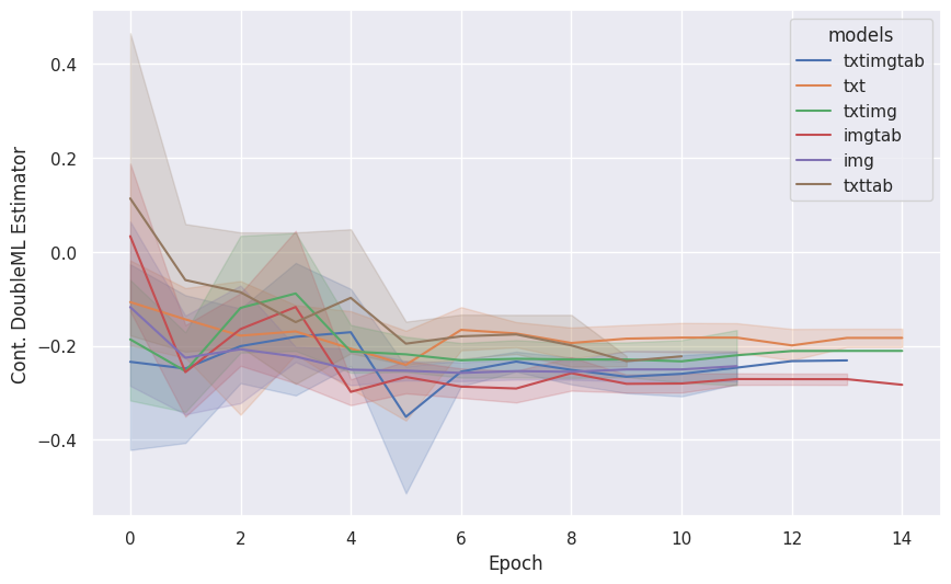
(First) Results

• Using different combinations of tabular, image and text data we obtain the following estimates

Continous Estimates from \(\texttt{DoubleMLPLR}\) on Validation Set during the Training Process

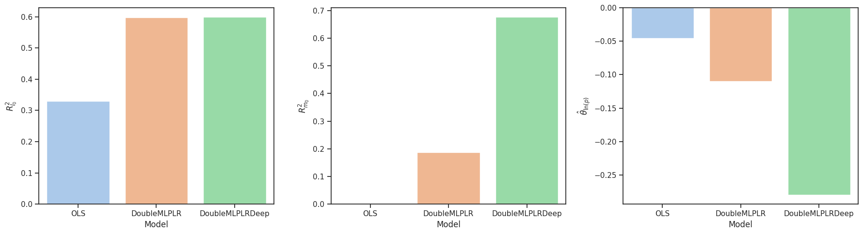
Comparison to Baseline Estimates

Model	Covariates	\(R^2_{l_0}\)	\(R^2_{m_0}\)	\(\hat{\theta}_0\)
\(\texttt{OLS}\)	\(X=X_{tab}\)	\(0.3300\)	-	\(-0.0455\)
\(\texttt{DoubleMLPLR}\)	\(X=X_{tab}\)	\(0.5986\)	\(0.1884\)	\(-0.1098\)
\(\texttt{DoubleMLPLRDeep}\)1	\(X=(X_{tab}, X_{txt}, X_{img})\)	\(0.5990\)	\(0.6765\)	\(-0.2794\)

1. Mean values of the \(\texttt{DoubleMLDeep}\) Model with tabular, text and image data as covariates.

More on Double Machine Learning

Papers & Book

• CausalML Book

• R package- with a nontechnical introduction to DML: Bach et al. (2021)

• Python package: Bach et al. (2022)

Software implementation:

• https://github.com/DoubleML/doubleml-for-py
• https://github.com/DoubleML/doubleml-for-r
• Docu and examples: docs.doubleml.org

Thank you!

GitHub Repository

If you like our package, you can leave us a ⭐ on GitHub

Contact

In case you have questions or comments, feel free to contact me

sven.klaassen@uni-hamburg.de

References

References

Bach, Philipp, Victor Chernozhukov, Malte S Kurz, and Martin Spindler. 2021. “DoubleML – An Object-Oriented Implementation of Double Machine Learning in R.” https://arxiv.org/abs/2103.09603.

———. 2022. “DoubleML-an Object-Oriented Implementation of Double Machine Learning in Python.” Journal of Machine Learning Research 23: 53–51.

Bajari, Patrick, Zhihao Cen, Victor Chernozhukov, Manoj Manukonda, Suhas Vijaykumar, Jin Wang, Ramon Huerta, et al. 2023. “Hedonic Prices and Quality Adjusted Price Indices Powered by AI.” https://arxiv.org/abs/2305.00044.

Chernozhukov, Victor, Denis Chetverikov, Mert Demirer, Esther Duflo, Christian Hansen, Whitney Newey, and James Robins. 2018. “Double/Debiased Machine Learning for Treatment and Structural Parameters.” The Econometrics Journal 21 (1): C1–68. https://onlinelibrary.wiley.com/doi/abs/10.1111/ectj.12097.

Ke, Guolin, Qi Meng, Thomas Finley, Taifeng Wang, Wei Chen, Weidong Ma, Qiwei Ye, and Tie-Yan Liu. 2017. “Lightgbm: A Highly Efficient Gradient Boosting Decision Tree.” Advances in Neural Information Processing Systems 30: 3146–54.

Krizhevsky, Alex. 2009. “Learning Multiple Layers of Features from Tiny Images.”

Maas, Andrew L., Raymond E. Daly, Peter T. Pham, Dan Huang, Andrew Y. Ng, and Christopher Potts. 2011. “Learning Word Vectors for Sentiment Analysis.” In Proceedings of the 49th Annual Meeting of the Association for Computational Linguistics: Human Language Technologies, 142–50. Portland, Oregon, USA: Association for Computational Linguistics. http://www.aclweb.org/anthology/P11-1015.

Wickham, Hadley. 2016. Ggplot2: Elegant Graphics for Data Analysis. Springer-Verlag New York. https://ggplot2.tidyverse.org.

Appendix

Amazon Toys Dataset

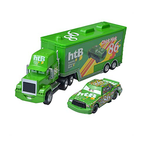
Data Examples

Kinsmart Set of 4 McLaren 720s Toy | …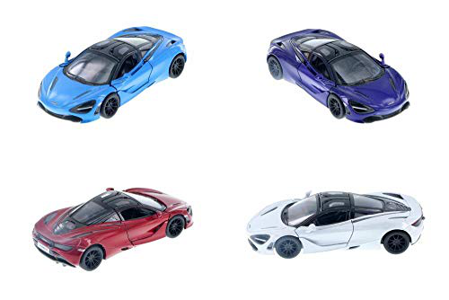

Pixar Cars Mack Uncle Lightning…

Neyman Orthogonality

The naive approach minimizes the following MSE

\[\begin{align} min_{\theta} \mathbb{E}[(Y - D\theta_0 - g_0(X))^2] \end{align}\]

This implies the following moment equation

\[\begin{align} \mathbb{E}[\underbrace{(Y - D\theta_0 - g_0(X))D}_{=:\psi (W, \theta_0, \eta)}]&=0 \end{align}\]

Whereas for the partialling-out approach minimizes

\[\begin{align} min_{\theta} \mathbb{E}\big[\big(Y - \mathbb{E}[Y|X] - (D-\mathbb{E}[D|X])\theta\big)^2\big] \end{align}\]

which implies

\[\begin{align} \mathbb{E}\big[\underbrace{\big(Y - \mathbb{E}[Y|X] - (D-\mathbb{E}[D|X])\theta\big)(D-\mathbb{E}[D|X])}_{=:\psi (W, \theta_0, \eta)}\big]&=0 \end{align}\]

Neyman Orthogonality

Naive approach

\[\begin{align} \psi (W, \theta_0, \eta) = & (Y - D\theta_0 - g_0(X))D \end{align}\]

Regression adjustment score

\[\begin{align} \eta &= g(X), \\ \eta_0 &= g_0(X). \end{align}\]

FWL partialling out

\[\begin{align} \psi (W, \theta_0, \eta_0) = & \Big((Y- E[Y|X])\\ &-(D-E[D|X])\theta_0\Big)\\ & (D-E[D|X]) \end{align}\]

Neyman-orthogonal score (Frisch-Waugh-Lovell)

\[\begin{align} \eta &= (\ell(X), m(X)), \\ \eta_0 &= ( \ell_0(X), m_0(X)), \\ &= ( \mathbb{E} [Y \mid X], \mathbb{E}[D \mid X]). \end{align}\]

DML Key Ingredients

1. Neyman Orthogonality

• Inference is based on a moment condition that satisfies the Neyman orthogonality condition \(\psi(W; \theta, \eta)\) \[E[\psi(W; \theta_0, \eta_0)] = 0,\]

• where \(W:=(Y,D,X,Z)\) and with \(\theta_0\) being the unique solution that obeys the Neyman orthogonality condition \[\left.\partial_\eta \mathbb{E}[\psi(W; \theta_0, \eta)] \right|_{\eta=\eta_0} = 0.\]

• \(\partial_{\eta}\) denotes the pathwise (Gateaux) derivative operator

DML Key Ingredients

1. Neyman Orthogonality

• Neyman orthogonality ensures that the moment condition identifying \(\theta_0\) is insensitive to small pertubations of the nuisance function \(\eta\) around \(\eta_0\)

• Using a Neyman-orthogonal score eliminates the first order biases arising from the replacement of \(\eta_0\) with a ML estimator \(\hat{\eta}_0\)

• PLR example: Partialling-out score function \[\psi(\cdot)= (Y-E[Y|X]-\theta (D - E[D|X]))(D-E[D|X])\]

DML Key Ingredients

2. High-Quality Machine Learning Estimators

• The nuisance parameters are estimated with high-quality (fast-enough converging) machine learning methods.

• Different structural assumptions on \(\eta_0\) lead to the use of different machine-learning tools for estimating \(\eta_0\) Chernozhukov et al. (2018) (Section 3)

• Rate requirements depend on the causal model and orthogonal score, e.g. (see Chernozhukov et al. (2018)),

  • PLR, partialling out: \(\lVert \hat{m}_0 - m_0 \rVert_{P,2} \times \big( \lVert \hat{m}_0 - m_0 \rVert_{P,2} + \lVert \hat{\ell}_0 - \ell_0\rVert _{P,2}\big) \le \delta_N N^{-1/2}\)
  • IRM/DR score, ATE: \(\lVert \hat{m}_0 - m_0 \rVert_{P,2} \times \lVert \hat{\ell}_0 - \ell_0\rVert _{P,2} \le \delta_N N^{-1/2}\)

DML Key Ingredients

3. Sample Splitting

• To avoid the biases arising from overfitting, a form of sample splitting is used at the stage of producing the estimator of the main parameter \(\theta_0\).

• Efficiency gains by using cross-fitting (swapping roles of samples for train / hold-out)

DML Key Ingredients

Main result in Chernozhukov et al. (2018)

There exist regularity conditions, such that the DML estimator \(\tilde{\theta}_0\) concentrates in a \(1/\sqrt{N}\)-neighborhood of \(\theta_0\) and the sampling error is approximately \[\sqrt{N}(\tilde{\theta}_0 - \theta_0) \sim N(0, \sigma^2),\] with \[\begin{align}\begin{aligned}\sigma^2 := J_0^{-2} \mathbb{E}(\psi^2(W; \theta_0, \eta_0)),\\J_0 = \mathbb{E}(\psi_a(W; \eta_0)).\end{aligned}\end{align}\]

• See this example based on Chernozhukov et al. (2018)